How To Copy Unique Values In Excel

Author: Oscar Cronquist Article last updated on September 27, 2021

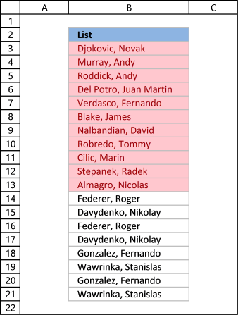
First, let me explain the divergence between unique values and unique singled-out values, it is important you know the difference so you can find the data you are looking for on this spider web page.

The moving-picture show above shows a list of values in column B, notation value AA has a duplicate. Unique distinct values are all jail cell values but duplicate values are merged into one distinct value. In other words, duplicates are removed only ane instance of each value is left in the list.

Column F contains unique values from column B, meaning values that exist only one time in cavalcade B. Value AA is not in column F because information technology has a indistinguishable, in other words, AA is not unique in column B. To filter duplicates, read this postal service: Extract a list of duplicates from a cavalcade

Table of Contents

Working with unique singled-out values

1. How to extract unique distinct values from a cavalcade [Formula]
   1. Video
   2. Copy unique distinct values
   3. Explaining formula
   4. Get Excel file
2. Extract unique distinct values (case sensitive) [Formula]
   1. Video
   2. Explaining formula
   3. Get Excel file
3. Filter unique distinct values [Avant-garde Filter]
   1. Video
   2. Copy unique singled-out values to another location
   3. Filter unique singled-out values, in place
4. Highlight unique distinct values [Conditional Formatting]
   1. Video
   2. Explaining formula
   3. Sort Conditional formatted cells at the elevation
5. How to hide duplicate values [Conditional Formatting]
6. Put unique singled-out values at the top of the list [Provisional Formatting]
7. Extract unique singled-out sorted values from a prison cell range [UDF]
   1. Video
   2. How to create an assortment formula
   3. VBA code
   4. Where to put the code?
8. Filter unique singled-out values from multiple sheets [Add together-In]
   1. Video
9. How to extract unique distinct values from a column [Onetime assortment Formula]
   1. How to create an assortment formula
   2. Explaining formula

Extract unique distinct values - Pivot Table (Link)

Working with unique values

1. 1. 10. How to filter unique values from a listing [Formula]
          1. Explaining formula
          2. Go Excel file
      11. Highlight unique values [Conditional Formatting]
          1. Video
          2. Sort unique values at the acme

Tips and tricks

1. 12. Useful tips
       1. Excel defined tables
       2. Named ranges
   13. Remove errors, Excel version 2007 and later
   14. Remove errors, Excel version 2003 and before
   15. How to ignore blank cells
       1. Video
       2. Get Excel file

• What you lot volition learn in this article
• What is possible with formulas?
• What is the easiest way to filter unique singled-out values?

What you will learn in this commodity

• The departure between unique distinct values and unique values.
• How to make up one's mind which Excel characteristic to use.
• How to utilize a formula that extracts unique distinct values.
  • How to copy the values returned by the formula.
  • How the formula works and the functions being used.
• How to filter unique distinct values because lowercase and uppercase letters.
• How to filter unique distinct values using the Advanced Filter.
• How to highlight unique distinct values using Provisional Formatting.
• How to build a User defined Office that filters unique distinct values sorted from A to Z.
  • Where to put the VBA lawmaking.
  • How to enter and apply the User defined Function.
• How to filter unique values using a formula.
• How to highlight unique values using Provisional Formatting.

Back to top

What is possible with formulas?

Y'all have quite a few options to cull from if you are looking for a manner to create a unique distinct listing in your workbook, all demonstrated in this post or on this website. Not only an exceptionally small regular formula, if you want to utilize that, but also awesome congenital-in features in Excel that makes your work so much easier.

Formulas are very versatile, they permit you to build solutions for very specific tasks similar filtering unique distinct values from 2 separate columns or three. If your list contains blanks and so this article is for you: Excerpt a unique singled-out listing and remove blanks

Mayhap you desire to practise a wildcard lookup and return unique distinct values or simply render unique distinct values based on a status.

I have also written manufactures that explains how to create a unique distinct list sorted alphabetically, sum or frequency.

At that place is also a formula for extracting unique singled-out values located in a multi-column cell range, information technology is a somewhat more complicated array formula, however, at that place is a custom function likewise, if yous prefer that.

Dorsum to top

What is the easiest mode to filter unique singled-out values?

I would cull the advanced filter if y'all are not looking for a formula. It lets you lot apace filter a unique singled-out list.

If you know that you will be extracting unique distinct values from time to time, similar in a dashboard or an interactive worksheet, I recommend using a formula and an Excel defined table. You won't need to repeat the same steps over and over compared to the advanced filter and that volition save you time and repetitive piece of work.

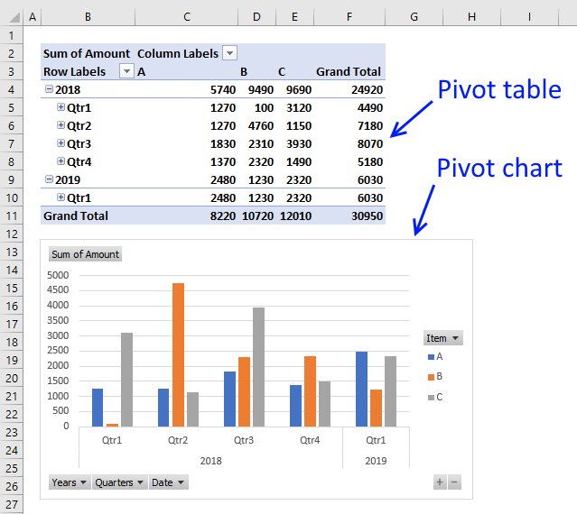
Nevertheless working with a large data gear up may tiresome down the formula calculations considerably depending on your estimator hardware, and so perhaps the User Defined Function [UDF] is a better choice or fifty-fifty ameliorate a pivot table, if yous accept huge amounts of information to work with.

The Excel Pivot tabular array is lightning fast even with huge data tables but it does take a little learning curve and it requires a few steps to set it up but in my opinion, information technology is totally worth learning how to utilize pivot tables. Y'all will be surprised how piece of cake it is to start working with Excel Pivot tables.

Conditional Formatting allows you to format cells determined by a built-in rule or a formula you construct. In this mail, you volition find a Conditional Formatting formula that highlights unique and unique distinct values. Did you lot know that you can easily sort highlighted values on superlative? Bank check out conditional formatting.

I take made an add-in that lets you extract unique, unique distinct and duplicate values and records from multiple worksheets. This allows you to hands bring together data from multiple sources in your workbook.

There is likewise a useful array formula in this article that extracts a case-sensitive unique distinct listing, this is a special case which the built-in Excel tools tin can't achieve.

Back to top

1. Create a listing of unique distinct values

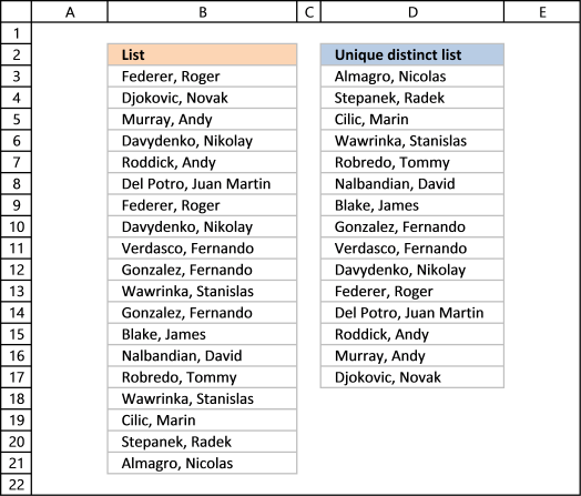
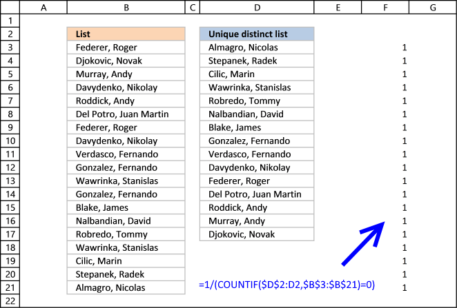
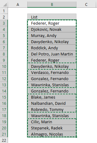
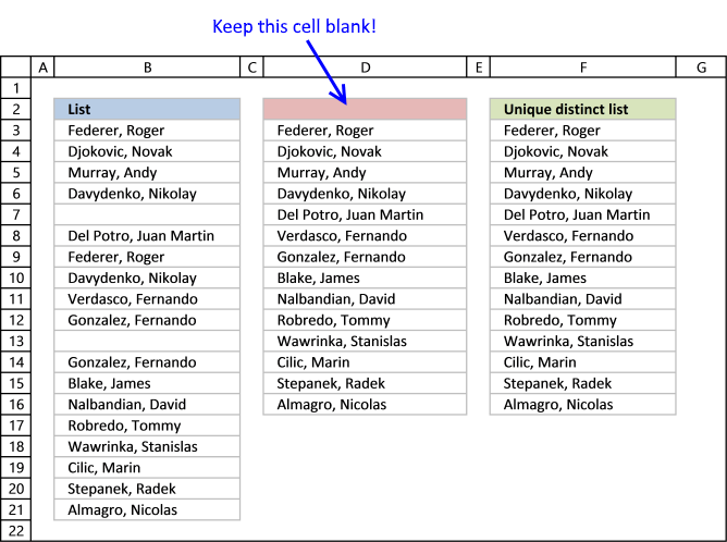
Column B contains names, some cells have duplicate values.  A formula in column D extracts a unique distinct list from column B.

Update: 2017-08-xv!

This formula is even smaller than the array formula and you lot are non required to enter this as an array formula. The following formula is for older Excel versions than Excel 365 subscribers.

Formula in cell D3:

=LOOKUP(ii,i/(COUNTIF($D$2:D2,$B$3:$B$21)=0),$B$3:$B$21)

I volition explain how this formula works in the video below and in section 1.3 also below.

Back to top

Update: 2020-05-28!

Microsoft Excel released new functions for Excel 365 subscribers in January 2020. One of those new functions is the UNIQUE function, information technology allows you to easily extract a unique distinct list using simply one part.

Formula in cell D3:

=UNIQUE(B3:B21)

This formula is entered as a regular formula, nevertheless, it is a dynamic array formula. Microsoft Excel introduced dynamic assortment formulas in January 2020 besides.

Dynamic array formulas expand to cells below automatically if more than one value is returned from the formula. Microsoft Excel calls this behavior spilling. You tin can find more case of the UNIQUE function here.

I will depict a formula for older Excel versions beneath.

Extract unique distinct values - Excel 365 (Link)
Extract unique singled-out values sorted from A to Z - Excel 365 (Link)
Extract unique distinct values ignoring blanks - Excel 365 (Link)
Excerpt unique distinct values sorted from A to Z ignoring blanks - Excel 365 (Link)

ane.1 Video

This video demonstrates how to employ the formula:

Subscribe to Go Digital Aid on Youtube:

Back to top

ane.2 Copy unique singled-out values

To re-create unique distinct values to some other location you lot must brand sure yous copy the values and not the formula:

1. Select list
2. Re-create list, shortcut keys: CTRL + C or press this push:
3. Printing with right mouse push on on destination prison cell and press with left mouse push button on the black arrow adjacent to "Paste Special..."
   
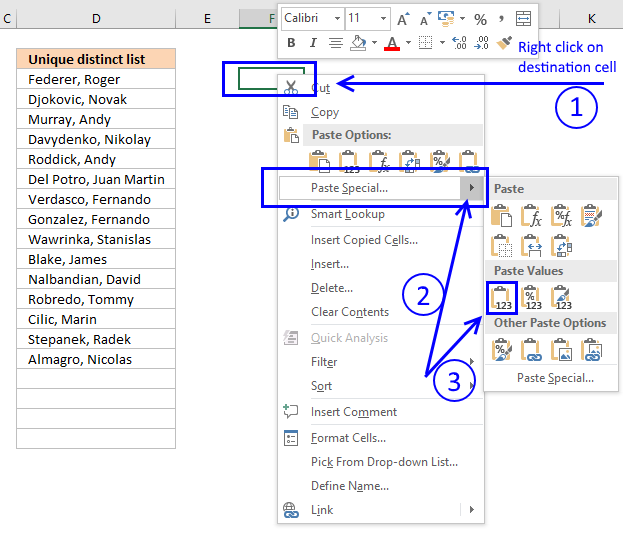
4. Then press with left mouse button on "Paste Values" button.

Dorsum to pinnacle

1.iii Explaining formula in cell D3

Step 1 - Count previous values to a higher place the electric current cell

The COUNTIF part allows yous to count values based on a condition. With the aid from an expanding cell reference, the formula knows which of the values that accept been extracted.

In cell D3 no values take been extracted so it compares the value in the cell above current cell, this happens to exist the Header value. Make sure yous don't have a value in the listing that matches the header value, it won't be extracted.

COUNTIF($D$ii:D2,$B$3:$B$21) is entered in column F, displayed in the film below.

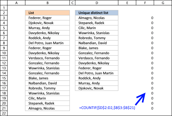
The value in cell D2 is non found in any instance in cell range B3:B21, all values in the array are 0 (nil). Note that the array has the same size as the list in column B, 19 values.

Step 2 - Compare array with 0 (zero)

To identify values that accept not been shown the formula compares the array with 0 (zero) and the event are boolean values (True or FALSE) for each value in the array.

COUNTIF($D$two:D2,$B$3:$B$21) = 0

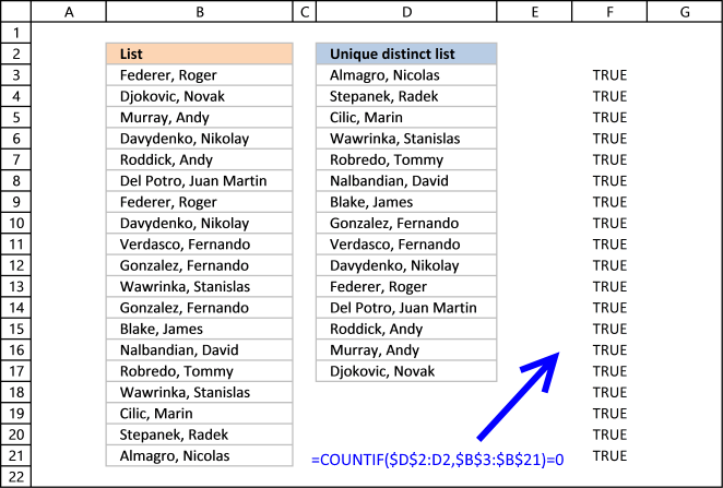
The array contains xix boolean values, all TRUE.

Step 3 - Divide 1 with assortment

The boolean value True is equal to 1 and Simulated is equal to 0. If a value in the assortment is Truthful the result will exist 1 because ane/True equals ane.

If a value in the array is Imitation the result volition be #DIV0! considering 1/FALSE is ane/0 and you can't divide a number with zero. Excel returns an fault.

The good matter about the LOOKUP function is that information technology ignores errors, encounter next stride.

Stride four - LOOKUP value

The LOOKUP function is designed to piece of work with sorted cell ranges or arrays, you get weird results if they are not sorted. Exist careful using the LOOKUP function.

Withal, in this case, the values in the array are either 1 or #DIV0!. Surprisingly information technology ignores errors, the only thing it tin find then is a value that is 1.

The beginning statement in the LOOKUP role is 2 so the part finds the last largest value that is equal to two or smaller.

LOOKUP(2,1/(COUNTIF($D$2:D2,$B$3:$B$21)=0),$B$iii:$B$21)

becomes

LOOKUP(2,{1;ane;1;i;1;i;1;one;i; 1;1;1;1;1;1;i;one;1;1},$B$iii:$B$21) and matches the last value in the array. LOOKUP function then returns the corresponding value in jail cell range $B$three:$B$21 which is Almagro, Nicolas

Back to top

1.4 Excel file

Extract a unique distinct list sorted from A to Z
Extract a unique distinct listing sorted from A to Z ignore blanks
Vlookup – Render multiple unique distinct values
Unique distinct list sorted alphabetically based on a condition
Extract a unique distinct listing from 2 columns
Excerpt a unique distinct list from three columns
Filter unique distinct records

Back to top

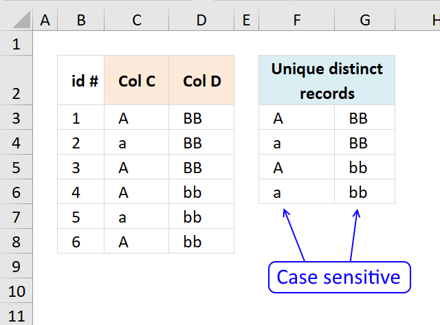
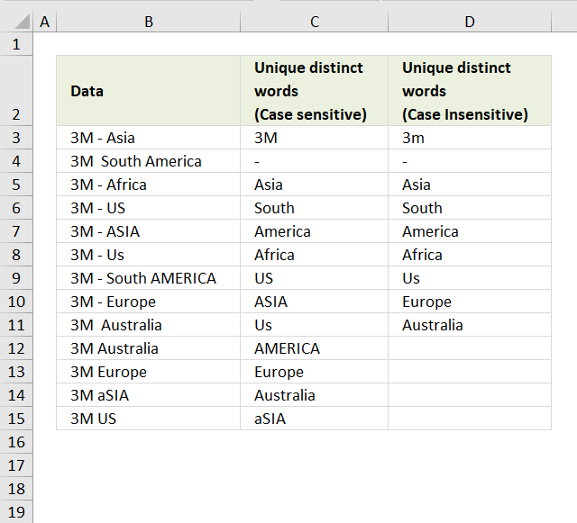
2. Extract a unique distinct listing (example sensitive)

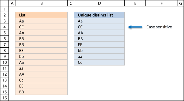
The following array formula lists unique singled-out values from a list also considering upper and lower letters. For case, the value "Aa" is non equal to "AA".

Array formula in prison cell D3:

=Alphabetize($B$3:$B$15, Lucifer(0, FREQUENCY(IF(Verbal($B$three:$B$15, TRANSPOSE($D$2:D2)), Lucifer(ROW($B$3:$B$fifteen), ROW($B$3:$B$xv)), ""), MATCH(ROW($B$3:$B$fifteen), ROW($B$three:$B$xv))), 0))

Excel 365 subscribers can use this regular somewhat shorter formula in cell D3 than the formula below:

=Permit(z, B3:B15, x, SEQUENCE(z), INDEX(z, MATCH(0, FREQUENCY(IF(EXACT(z, TRANSPOSE($D$2:D2)), x, ""), x), 0))

The formula above contains ii new formulas: Permit office and the SEQUENCE function.

This commodity explains the formula: Excerpt a case sensitive unique list from a cavalcade - Excel 365

2.1 Video

This video demonstrates how to build a formula that extracts a case-sensitive unique distinct listing:

Subscribe to Get Digital Help on Youtube:

This post shows you how to extract a case sensitive unique listing from a column:

How to extract a case sensitive unique list from a cavalcade

How to enter an array formula

Back to top

ii.2 Explaining the assortment formula in cell C3

Pace 1 - Transpose previous values

TRANSPOSE($D$2:D2)

becomes

TRANSPOSE({"Unique distinct list (case sensitive)";"Aa"})

and returns

{"Unique distinct list (case sensitive)","Aa"}

Note that the ; (semicolon) changes to a , (comma)

Recommended reading:

How to use the TRANSPOSE function

Step 2 - Check if two text strings are exactly the same, also instance sensitive

Verbal($B$3:$B$xv, TRANSPOSE($D$two:D2))

becomes

Verbal($B$3:$B$15, TRANSPOSE({"Unique singled-out list (case sensitive)","Aa"})

becomes

Verbal($B$3:$B$15, TRANSPOSE({"Unique singled-out list (case sensitive)","Aa"})

becomes

EXACT({"Aa"; "CC"; "AA"; "BB"; "BB"; "EE"; "bb"; "Aa"; "aa"}, TRANSPOSE({"Unique distinct list (case sensitive)","Aa"})

and returns

{Fake, Truthful; FALSE, FALSE; FALSE, Faux; Imitation, False; Fake, Simulated; FALSE, FALSE; FALSE, Simulated; Fake, TRUE; FALSE, FALSE}

Stride iii - Render relative position in array if Truthful

IF(Exact($B$3:$B$15, TRANSPOSE($C$1:C1)), Match(ROW($B$3:$B$15), ROW($B$three:$B$15))

becomes

IF({FALSE, TRUE; FALSE, Imitation; FALSE, FALSE; FALSE, FALSE; Fake, False; FALSE, FALSE; FALSE, FALSE; Simulated, TRUE; FALSE, FALSE}, MATCH(ROW($A$1:$A$9), ROW($A$i:$A$9)))

becomes

IF({Fake, TRUE; Fake, FALSE; Fake, FALSE; Imitation, False; FALSE, FALSE; Simulated, FALSE; FALSE, Simulated; FALSE, True; Fake, Fake}, {1;two;3;four;5;half-dozen;7;8;ix})

and returns

{Faux,1; Simulated,False; Faux,False; Fake,False; FALSE,FALSE; Faux,False; Imitation,Simulated; Simulated,8; Fake,False}

Recommended article:

How to use the COUNTIF function

Step 4 - Calculate how often values be in an array

FREQUENCY(IF(EXACT($B$3:$B$15, TRANSPOSE($C$ane:C1)), MATCH(ROW($B$3:$B$15), ROW($B$three:$B$15)), ""), MATCH(ROW($B$iii:$B$15), ROW($B$3:$B$fifteen)))

becomes

FREQUENCY({FALSE,one; Faux,Imitation; Imitation,FALSE; Imitation,FALSE; Fake,Simulated; FALSE,FALSE; Imitation,Faux; Fake,viii; Simulated,FALSE},Friction match(ROW($B$3:$B$fifteen),ROW($B$three:$B$15)))

becomes

FREQUENCY({False,ane; FALSE,FALSE; Faux,FALSE; Simulated,FALSE; Fake,Fake; False,FALSE; False,FALSE; FALSE,viii; Fake,Fake},{1;2;3;4;v;vi;7;eight;ix})

and returns

{i;0;0;0;0;0;0;1;0;0} Aa is found in position 1 and eight in cell range $B$three:$B$xv

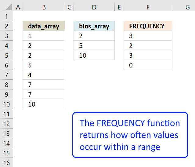
How to apply the FREQUENCY role

Step 5 - Discover first empty value (0) in array

MATCH(0, FREQUENCY(IF(EXACT($B$iii:$B$15, TRANSPOSE($C$i:C1)), Friction match(ROW($B$3:$B$xv), ROW($B$3:$B$fifteen)), ""), Lucifer(ROW($B$3:$B$fifteen), ROW($B$three:$B$fifteen))), 0)

becomes

MATCH(0, {1;0;0;0;0;0;0;ane;0;0}, 0)

and returns 2.

How to use the Friction match function

Stride 6 - Return value from position ii

Index($B$3:$B$15, MATCH(0, FREQUENCY(IF(EXACT($B$3:$B$15, TRANSPOSE($C$1:C1)), MATCH(ROW($B$3:$B$xv), ROW($B$three:$B$15)), ""), MATCH(ROW($B$3:$B$15), ROW($B$3:$B$fifteen))), 0))

becomes

Index($B$iii:$B$15, two)

and returns "CC" in jail cell C3.

How to apply the INDEX function

Dorsum to tiptop

2.3 Excel file

Back to top

Recommended articles

Instance sensitive lookup and return multiple values
Filter values based on a condition - case sensitive (Excel 365)
Filter unique singled-out values (case sensitive) [UDF]
Filter unique singled-out records (case sensitive) [UDF]

Dorsum to top

3. Extract unique distinct values [Avant-garde Filter]

Commencement a little reminder, unique distinct values are all cell values but duplicate values are merged into one distinct value.

three.1 Video

The following video shows you how to filter unique singled-out values using Advanced Filter:

Subscribe to Get Digital Help on Youtube:

Dorsum to top

3.ii Instructions - Copy unique distinct values to another location

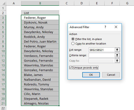
This section describes how to extract unique distinct values using the congenital-in feature "Advanced Filter".

1. Go to tab "Data" on the ribbon.
2. Press the "Advanced Filter" button on the ribbon.
   
   
3. Press push "Copy to some other location".
   
   
4. Press "List range:" and select range to filter unique distinct values.
5. Printing "Copy to: and select a range.
6. Press "Unique records only" button to select it.
7. Press with left mouse button on "OK" push button to apply settings and get-go extracting.

Back to top

3.3 Instructions - Filter unique singled-out values, in place

If y'all choose to filter unique singled-out values in-place, press with left mouse button on the get-go selection button in the dialog box.

Yous tin can then select unique distinct values and paste to another location, duplicate values are subconscious and are ignored when you copy cell range B3:21 and paste to a new location, very useful.

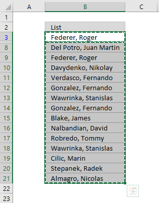
The film beneath shows you the selected distinct values after I cleared the Advanced Filter, duplicate values are non selected because they were hidden.

Recommended manufactures

Lookup and render multiple values [Avant-garde Filter]
Excerpt all rows that meet critera in 1 cavalcade [Advanced Filter]

An Advanced Filter is not the only powerful built-in feature in Excel, I highly recommend that you learn pin tables. Perhaps the about powerful tool but also the to the lowest degree known:

How to apply Pivot Tables – Excel's virtually powerful feature and also to the lowest degree known

The Excel defined table is also extremely useful, information technology allows yous to apace sort, filter and manipulate data. Larn that and much more:

How to use Excel Tables

An Excel table allows you to easily sort, filter and sum values in a data ready where values are related.

How to use Excel Tables

Back to top

This section demonstrates how to highlight unique distinct values using Excel's built-in feature "Conditional Formatting".

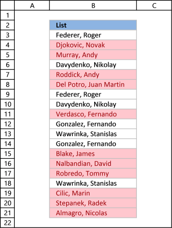
The image shows you unique distinct values highlighted using Provisional Formatting.

4.1 Video

This video demonstrates how to highlight unique distinct values:

Subscribe to Go Digital Assistance on Youtube:

How to highlight unique distinct values

1. Select cell range B3:B21.
2. Go to tab "Home" on the ribbon.
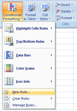
3. Press on "Conditional Formatting" button.
   
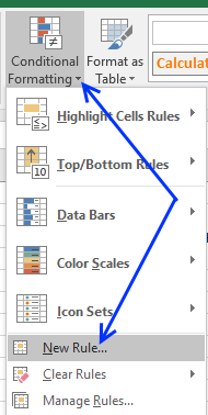
4. Press on "New Rule...".
   
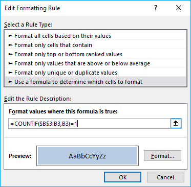
5. Press on "Use a formula to make up one's mind which cells to format:".
6. Type this formula: =COUNTIF($B$three:B3,B3)=1
7. Press on "Format..." button.
8. Pick a color.
9. Press OK push.
10. Press OK button again.

Back to superlative

4.2 Explaining Provisional Formatting formula

A CF formula works somewhat differently than a regular formula, even so, they may be harder to spot.

It is possible that y'all can't even run into if a cell range has CF applied to it or not, if no cells are highlighted.

I recommend that you copy the CF formula and enter information technology to an adjacent column to improve testify how they work.

Step 1 - COUNTIF office

The COUNTIF function has two arguments, the get-go argument is the cell range you desire to count a specific value in. The 2nd argument is the value you desire to count.

COUNTIF(range,criteria)

Step 2 - COUNTIF arguments

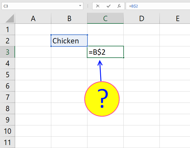
The first argument uses both relative and absolute cell references, $B$3:B3. The accented role has dollar signs $B$three meaning it does not change when the Conditional Formatting formula is applied to the adjacent cell.

The relative part B3 does change when the Conditional Formatting formula is applied to the next cell.

COUNTIF($B$3:B3, B3)

Footstep three - Demonstrate calculations in cells B3 and B4

In prison cell B3 the part is COUNTIF($B$iii:B3,B3)

and in prison cell B4: COUNTIF($B$3:B4,B4) and and then on.

This technique using growing cell references lets you highlight the starting time instance of a value but not duplicate values.

Stride 4 - Compare output to 1

How do we know if the value is a unique singled-out value? Compare COUNTIF($B$three:B3,B3) to 1 and information technology will return TRUE or Simulated, similar this:

COUNTIF($B$3:B3,B3)=one

The equal sign is a logical operator that returns TRUE or FALSE. Note, the comparison is not example sensitive. The output is a boolean value TRUE or Fake.

COUNTIF($B$three:B3,B3)=i

becomes

1=1

and returns boolean value True. Cell B3 is highlighted.

If COUNTIF($B$3:B3,B3) returns a number larger than 1 pregnant there is at least a indistinguishable value in the jail cell range specified in the first argument. That prevents the Conditional Formatting formula from highlighting the prison cell.

Recommended articles
Highlight unique/duplicates
Highlight current engagement
Highlight lookup values
Highlight cells equal to

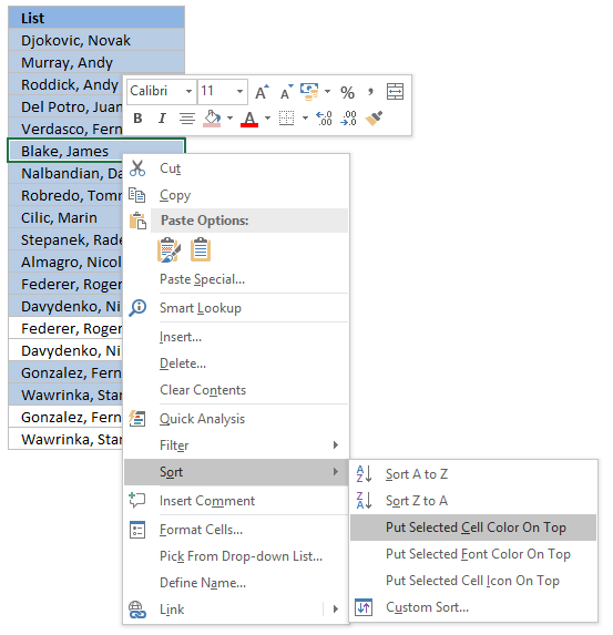
4.iii Sort Conditional formatted cells at the top

Tip! Press with correct mouse push on on a highlighted cell, press with left mouse button on Sort and then on "Put Selected Prison cell Colour On superlative" to conform unique distinct values at the very top of your list.

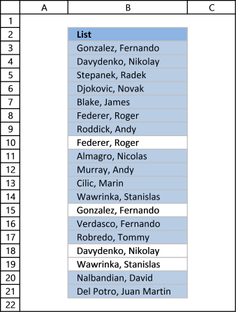
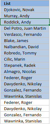
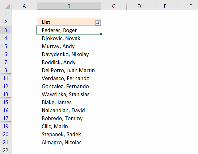
The picture show below shows you all unique singled-out values sorted together.

Back to top

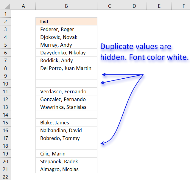
The image higher up demonstrates Provisional Formatting practical to a listing of values, it changes the font color to white for indistinguishable values making them invisible or they appear hidden.

Go along in mind that the text is still there and so if you lot copy the range and paste the values to a new range the subconscious values are visible again. I recommend that you lot sort the visible values at the elevation in guild to copy them correctly, instructions below.

Provisional Formatting formula:

=COUNTIF($B$3, B3)>one

Back to summit

How to apply conditional formatting formula to cell range B3:B21

1. Select cell range B3:B21.
2. Go to tab "Home" on the ribbon.
3. Press with left mouse button on the "Conditional Formatting" push button.
4. Press with left mouse push button on "New Rule..."
   
5. Printing with left mouse button on "Use a formula to decide which cells to format:".
   
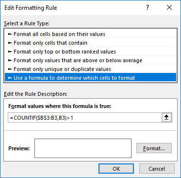
6. Type the Conditional Formatting formula in "Format values where this is true:".
7. Press with left mouse push button on "Format..." button.
   
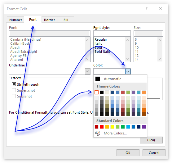
8. Go to tab "Font" on the menu, see image to a higher place.
9. Press with left mouse button on colour drib-down list.
10. Pick white.
11. Printing with left mouse push button on OK button.
12. Press with left mouse push button on OK button.
13. Press with left mouse button on OK button.

Dorsum to top

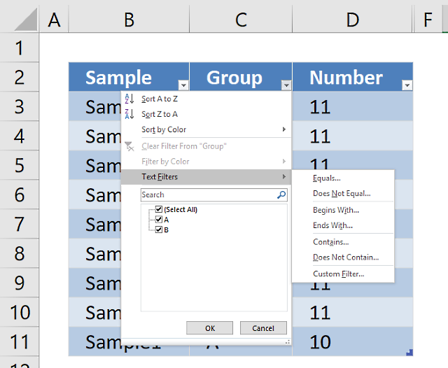
vi. How to sort unique distinct values at the top of the list

1. Press with right mouse button on on one of the visible values in the listing.
   
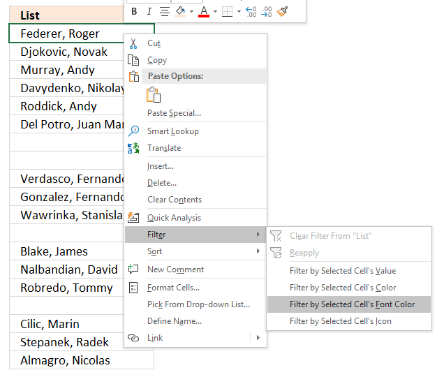
2. Printing with left mouse push on "Filter"
3. Printing with left mouse push on "Filter by Selected Cell's Font colour.

Recommended articles
Highlight unique values and unique distinct values in a multi-cavalcade jail cell range
Highlight unique singled-out records
Highlight unique values in a filtered excel table
How to highlight indistinguishable values in a column
Check out the Provisional formatting category

Back to top

7. Extract unique distinct sorted values from a prison cell range [UDF]

This UDF lets you create and sort a unique singled-out list. First y'all need to re-create the VBA lawmaking to your workbook, instructions below. Second, select a cell range. Third, type FilterUniqueSort(cell_ref) in the formula bar. Final, enter formula every bit an array formula, instructions below.

At that place is likewise a workbook for you to get.

Assortment formula in cell B2:B8212:

=FilterUniqueSort($A$2:$A$8212)

7.1 Video

This video explains how to implement and use the User Defined Function

Subscribe to Get Digital Help on Youtube:

seven.2 How to create an array formula

1. Type B2:B8212 in proper name box
2. Type above array formula in formula bar
   
3. Printing and concord Ctrl + Shift
4. Press Enter once
5. Release all keys

Recommended reading

A beginners guide to Excel array formulas

Back to top

seven.three VBA code

I am using the selection sort function to sort values. Yous can read more about the function here:

Using a Visual Basic Macro to Sort Arrays in Microsoft Excel

'Proper noun User Defined Role and ascertain paremeter Part FilterUniqueSort(rng As Range)  'Dimension variables and declare information types Dim ucoll Equally New Collection, Value As Variant, temp() Every bit Variant Dim iRows As Single, i As Unmarried  'Redimension array variable ReDim temp(0)  'Enable fault handling On Error Resume Next  'Iterate through each value in range For Each Value In rng  'Check if number of characters in value is greater than 0 (zero), if true add together value to collection ucoll If Len(Value) > 0 Then ucoll.Add Value, CStr(Value)  'Go on with next value Next Value  'Disable error handling On Error GoTo 0  'Iterate through each value in collection ucoll For Each Value In ucoll  'Save value to last container in array variable temp temp(UBound(temp)) = Value  'Add new container to array variable temp ReDim Preserve temp(UBound(temp) + ane)  'Next value Next Value  'Remove last container in array variable temp ReDim Preserve temp(UBound(temp) - i)  'Save selected rows on worksheet to variable iRows iRows = Range(Application.Caller.Accost).Rows.Count  'Get-go User Defined Function SelectionSort with values in array variable temp SelectionSort temp  'Add together blanks to array variable temp to forbid error values on worksheet For i = UBound(temp) To iRows  'Add container ReDim Preserve temp(UBound(temp) + 1)  'Save blank to container temp(UBound(temp)) = ""  'Continue with next value Next i  'Transpose values in array variable temp and return those values to worksheet FilterUniqueSort = Awarding.Transpose(temp)  End Office        

'Proper noun User Divers Office (UDF) and define parameters Function SelectionSort(TempArray Every bit Variant) 'This UDF sorts values in an array 'https://www.get-digital-assistance.com/how-to-extract-a-unique-list-and-the-duplicates-in-excel-from-one-column/#7.three            'Dimension variables and declare data types           Dim MaxVal Every bit Variant           Dim MaxIndex Equally Integer           Dim i As Integer, j As Integer                      'Iterate through each value in array variable temp starting from last to starting time           For i = UBound(TempArray) To 0 Step -i                'Save value to variable MaxVal               MaxVal = TempArray(i)                'Save value stored in variable i to variable MaxIndex               MaxIndex = i                'Iterate through each value in array variable temp               For j = 0 To i                    'Check if value in array variable TempArray is larger than value stored in variable MaxVal                   'Excel can compare text values besides, this action checks if a text value is earlier or later on another value in a sorted list                    If TempArray(j) > MaxVal Then                        'If true save value to variable MaxVal                       MaxVal = TempArray(j)                        'Relieve position to MaxIndex                       MaxIndex = j                   Terminate If                'Continue with next value               Next j                'Check if number stored in variable MaxIndex is smaller than number stored in variable i               If MaxIndex < i Then                    'Save value in assortment variable TempArray position i to assortment variable TempArray container position MaxIndex                   TempArray(MaxIndex) = TempArray(i)                    'Save value in variable MaxVal to array variable TempArray container position i                   TempArray(i) = MaxVal               End If           Side by side i        End Function        

Back to top

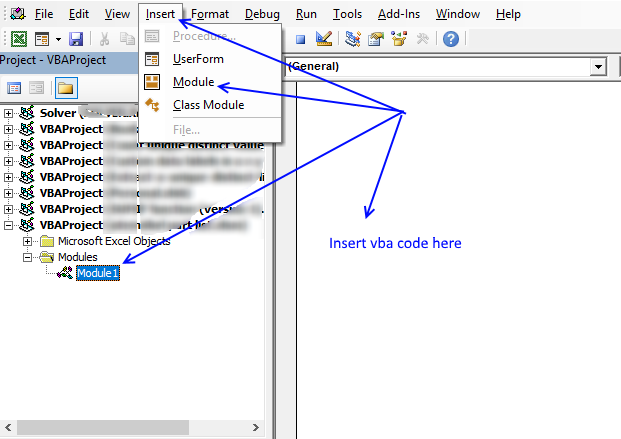
7.four Where to copy VBA code?

1. Printing Alt + F11 to open VB Editor
2. Press with left mouse button on "Insert" on the menu
3. Press with left mouse button on "Module" to create a module
4. Re-create (Ctrl + c) in a higher place VBA code and paste (Ctrl +v)  to the code module

Back to superlative

More than powerful User Defined Functions

Filter unique distinct records (case sensitive) [UDF]

Lookup and return multiple values concatenated into one cell

Filter unique distinct words from a cell range [UDF]

Back to meridian

8. Filter unique singled-out values from multiple sheets add-in

Filter unique distinct valuesis an add-in for Excel 2007/2010/2013 that lets yous excerpt

• unique distinct values
• duplicate values
• unique distinct records
• duplicate records

from multiple sheets. The Add-In contains 4 user-defined functions.

If a value in ane of the ranges changes the function will automatically and instantly update the list.

Features

• All user-defined functions remove blank values and blank records.
• No error values when all values are extracted.
• Filter values or records from up to 255 different cell ranges or sheets.

8.1 Watch this video where I demonstrate the Excel Add-In

Subscribe to Go Digital Assist on Youtube:

What are unique distinct values?

What are unique distinct records?

Purchase Filter Unique Distinct Values From Multiple Sheets Add-in For Excel 2007/2010/2013 - Price $xix USD

Questions

Is there a money back guarantee?
Sure, y'all have a unconditional coin back guarantee for 14 days.

Back to top

9. Create a listing of unique singled-out values [Old array Formula]

I recommend using the regular formula in a higher place since it is smaller and has an reward of not being an array formula.

Array formula in cell D3:

=Alphabetize($B$3:$B$21, Lucifer(0, COUNTIF($D$ii:D2, $B$three:$B$21), 0))

Thanks to Eero, who contributed the original array formula!

Back to meridian

The formulas above has an result with blank cells, it returns a 0 (nada) in your listing. This article shows you how to ignore blanks:

Extract a unique singled-out listing and ignore blanks

9.1 How to create an assortment formula

You don't demand to follow these steps if you chose the regular formula.

1. Copy the array formula to a higher place (Ctrl + c)
2. Double press with left mouse button on jail cell B2
3. Paste (Ctrl + 5)
4. Press and hold Ctrl + Shift simultaneously
5. Press Enter
6. Release all keys

If you lot made the above steps correctly the formula at present has a beginning and ending curly bracket, similar this:
{=INDEX($B$3:$B$21, MATCH(0, $D$ii:D2, $B$3:$B$21), 0))}

Don't enter these characters yourself, they appear automatically.

Re-create cell B2 and paste to cells below as far as needed.

Back to tiptop

9.2 How the array formula in cell B2 works

Step 1 - Create an assortment with the aforementioned size as the list

The COUNTIF office calculates the number of cells equal to a status.

COUNTIF(range,criteria)

COUNTIF($B$1:B1, $A$2:$A$20)

becomes

COUNTIF("Unique distinct list",{Federer,Roger; Djokovic,Novak; Murray,Andy; Davydenko,Nikolay; Roddick,Andy; DelPotro,JuanMartin; Federer,Roger; Davydenko,Nikolay; Verdasco,Fernando; Gonzalez,Fernando; Wawrinka,Stanislas; Gonzalez,Fernando; Blake,James; Nalbandian,David; Robredo,Tommy; Wawrinka,Stanislas; Cilic,Marin; Stepanek,Radek; Almagro,Nicolas} )

and returns:

{0;0;0;0;0;0;0;0;0;0;0;0;0;0;0;0;0;0;0}

This means the cell value in $B$one:B1 tin can't be found in whatever of the cells in cell range $A$ii:$A$20. If it had been found, somewhere in the array the number i would exist.

Stride 2 - Return the position  of an particular that matches 0 (zero)

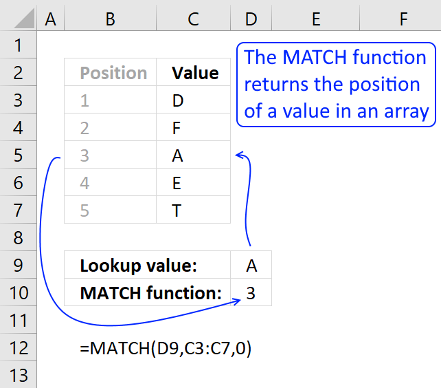
The Friction match function returns the relative position of an detail in an assortment that matches a specified value.

Lucifer(lookup_value, lookup_array, [match_type]

Lucifer(0, COUNTIF($B$ane:B1, $A$2:$A$twenty), 0)

becomes

MATCH(0,{0; 0; 0; 0; 0; 0; 0; 0; 0; 0; 0; 0; 0; 0; 0; 0; 0; 0; 0},0)

and returns ane.

Footstep three - Return a prison cell value

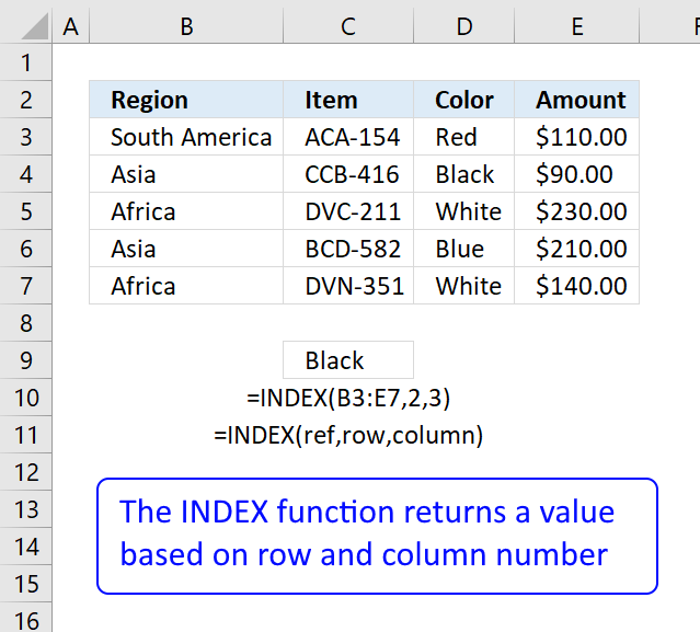
The Index role returns a value or reference of the cell at the intersection of a particular row and column, in a given range.

Alphabetize(array, row_num, [column_num])

Alphabetize($B$three:$B$21, 1)

becomes

=Alphabetize({Federer,Roger; Djokovic,Novak; Murray,Andy; Davydenko,Nikolay; Roddick,Andy; DelPotro,JuanMartin; Federer,Roger; Davydenko,Nikolay; Verdasco,Fernando; Gonzalez,Fernando; Wawrinka,Stanislas; Gonzalez,Fernando; Blake,James; Nalbandian,David; Robredo,Tommy; Wawrinka,Stanislas; Cilic,Marin; Stepanek,Radek; Almagro,Nicolas}, 1)

and returns "Federer, Roger".

Relative and absolute cell references

When you copy the array formula downwards the countif formula range ($B$1:B1) expands. This is created by using relative and absolute references.

The commencement cell, B2: COUNTIF($B$1:B1,$A$two:$A$20)

2nd cell, B3: COUNTIF($B$1:B2,$A$two:$A$xx)

and so on.

Recommended reading:

How to utilise absolute and relative references

Back to height

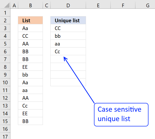
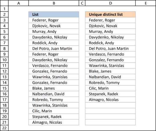
10. How to filter unique values from a listing

Unique values are values existing only in one case in a list. Case, "AA" exists twice in the list beneath and is not unique. BB and CC be only in one case each and are unique in the list.

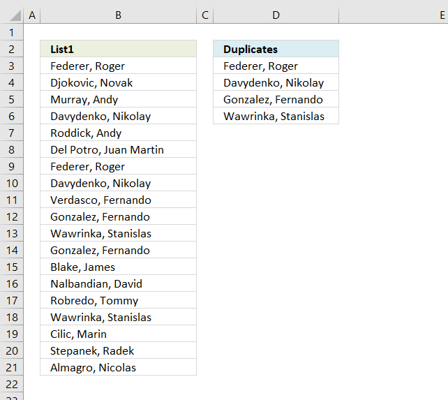
Column D in the picture below filters all unique values from column B. Unique values are values that exist but once in column B.

Instance, Roger, Federer is not in cavalcade D because there is more than than one value of this name in column A. In other words, the name is non unique in cavalcade A. You lot tin can detect the proper noun twice in the list, in cells A2 and A8.

Update 2017-08-thirty
This formula is even smaller than the assortment formula and you lot are not required to enter this every bit an array formula.

Regular formula in jail cell D3:

=LOOKUP(two, ane/((COUNTIF(D2:$D$two, $B$3:$B$21)=0)*(COUNTIF($B$3:$B$21, $B$iii:$B$21)=ane)), $B$3:$B$21)

Recommended articles

How to extract a case sensitive unique list from a cavalcade
Filter unique values sorted from A to Z
Excerpt unique values from ii columns

Update 2020-12-09, the formula below extracts unique values from prison cell range $B$3:$B$21:

Regular formula in cell D3:

=UNIQUE($B$3:$B$21,,Truthful)

The formula above contains the new UNIQUE function that only Excel 365 subscribers tin can use. Use the formula higher up if you have an before Excel version.

Recommended articles

Excerpt unique values - Excel 365 (Link)
Extract unique values sorted from A to Z - Excel 365 (Link)
Extract unique values ignoring blanks - Excel 365 (Link)
Extract unique values sorted from A to Z ignoring blanks - Excel 365 (Link)

Array formula in cell D3:

=INDEX($B$3:$B$21, Match(0, COUNTIF(D2:$D$2, $B$3:$B$21)+(COUNTIF($B$3:$B$21, $B$three:$B$21)<>1), 0))

How to enter an array formula

Dorsum to top

10.1 Explaining array formula in cell D3

Step ane - Count each value in array and cheque if it is not equal to 1

(COUNTIF($A$ii:$A$20, $A$2:$A$20)<>1

becomes

{2;1;1;2;1;1;2;2;one;2;2;2;i;one;1;2;one;1;ane}<>one

and returns

{True; Simulated; False; Truthful; Imitation; Simulated; Truthful; True; Fake; Truthful; TRUE; TRUE; Fake; False; FALSE; TRUE; Faux; Simulated; FALSE}

This assortment tells excel that the start value in the array is not unique and that is true because Roger, Federer is not unique in the list. All the same the 2d value is Imitation and that value is unique, etc.

How to use the COUNTIF function

Step 2 - Go on track of previous values

C1:$C$1 is a dynamic cell reference, it changes as the formula is copied to cells below. You lot tin can read more than about absolute and relative cell references here:

How to employ absolute and relative references

COUNTIF(C1:$C$1, $A$two:$A$20)

becomes

COUNTIF("Unique list", {"Federer, Roger "; "Djokovic, Novak "; "Murray, Andy "; "Davydenko, Nikolay "; "Roddick, Andy "; "Del Potro, Juan Martin "; "Federer, Roger "; "Davydenko, Nikolay "; "Verdasco, Fernando "; "Gonzalez, Fernando "; "Wawrinka, Stanislas "; "Gonzalez, Fernando "; "Blake, James "; "Nalbandian, David "; "Robredo, Tommy "; "Wawrinka, Stanislas "; "Cilic, Marin "; "Stepanek, Radek "; "Almagro, Nicolas "})

and returns

{0; 0; 0; 0; 0; 0; 0; 0; 0; 0; 0; 0; 0; 0; 0; 0; 0; 0; 0}

A zilch (0) means that no values have nonetheless been displayed and that is true in cell C2. However when excel calculates the value in jail cell C3, prison cell C2 shows "Djokovic, Novak" and the assortment becomes {0; ane; 0; 0; 0; 0; 0; 0; 0; 0; 0; 0; 0; 0; 0; 0; 0; 0; 0}. The second value in the array contains ane. This tells excel that value has already been shown.

Step 3 - Add together arrays

COUNTIF(C1:$C$1, $A$ii:$A$20)+(COUNTIF($A$2:$A$20, $A$2:$A$20)<>1

becomes

{TRUE; FALSE; Fake; Truthful; Faux; Fake; True; True; FALSE; True; True; TRUE; FALSE; Imitation; Simulated; TRUE; FALSE; False; FALSE} + {0; 0; 0; 0; 0; 0; 0; 0; 0; 0; 0; 0; 0; 0; 0; 0; 0; 0; 0}

and returns

{1;0;0;1;0;0;1;ane;0;one;ane;1;0;0;0;1;0;0;0}

TRUE is 1 and FALSE is zero. So True + 0 equals i and False + 1 equals 1.

Step 4 - Detect kickoff aught value in array

A zero in the array indicates {ane;0;0;1;0;0;1;1;0;ane;1;1;0;0;0;ane;0;0;0} that the corresponding value is unique and has not still been displayed in the list.

Match(0, COUNTIF(C1:$C$1, $A$2:$A$20)+(COUNTIF($A$2:$A$twenty, $A$2:$A$20)<>one), 0)

becomes

MATCH(0, {1;0;0;1;0;0;one;1;0;1;1;1;0;0;0;i;0;0;0}, 0)

and returns 2.

How to utilize the Match function

Step 5 - Return respective value

Index($A$2:$A$20, Friction match(0, COUNTIF(C1:$C$1, $A$2:$A$20)+(COUNTIF($A$2:$A$twenty, $A$2:$A$20)<>1), 0))

becomes

INDEX($A$two:$A$20, 2)

and returns "Djokovic, Novak" in cell C2.

How to employ the Index function

Dorsum to tiptop

10.2 Get Excel file

To extract duplicates, come across this mail:

Extract a list of duplicates from a column

Dorsum to acme

eleven. Highlight unique values [Conditional Formatting]

This example demonstrates how to highlight cells with a color of your choice if it contains a unique value.

11.ane Video

The post-obit video shows you how to color unique values using conditional formatting. Remember, it highlights only unique values, in other words, values that exist simply one time in the listing.

Subscribe to Become Digital Help on Youtube:

Instructions

1. Get to tab "Home" on the ribbon
   
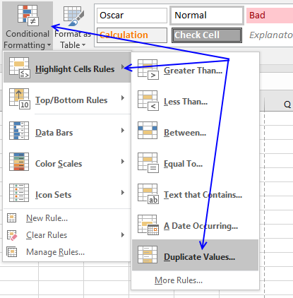
2. Press with left mouse button on "Provisional Formatting" button
3. Hover over "Highlight Cell Rules"
4. Printing with mouse on "Duplicate Values..."
   
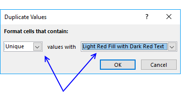
5. Press with mouse on the leftmost drop-downward listing and modify it to "Unique"
6. Option a formatting if you similar
7. Printing with left mouse button on OK button

The picture above shows you, for example, that the first name in the list has a duplicate so that proper name is not highlighted in any prison cell.

xi.2 Sort unique values at the top

Tip! Did you lot know that y'all tin can put highlighted values to the top

1. Press with correct mouse push on on a highlighted jail cell
   
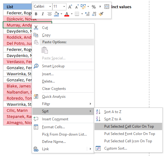
2. Printing with mouse on "Sort"
3. Printing with mouse on "Put Selected Cell Colour On Peak"

Back to acme

12. Useful tips

12.i Excel tables

An Excel Tabular array is a great feature and is very cleverly designed. Information technology is synthetic to automatically expand if you add more data which is incredibly helpful. You don't need to practise anything, not adjusting cell references which is fourth dimension consuming and prone to errors.

Structured references are cell references to an excel defined tabular array. They let you hands run into what the data contains as long every bit you give it good descriptive column header names.

I recommend you apply excel defined tables instead of named ranges or dynamic named ranges as long equally you lot are working with more 1 value.

Here is how to convert a list to an excel divers table:

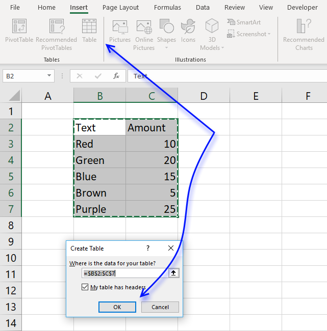
1. Select a prison cell in your list
2. Go to tab "Insert" on the ribbon and press with left mouse button on Table button or press Ctrl + T
3. Press with left mouse button on OK button
4. Your excel defined table is created

Read more about excel defined tables

Dorsum to top

12.two Named ranges

In excel you can name a cell range, a abiding or a formula. You can so use the named range in a formula, making information technology easier for you to read and understand formulas.

Example

List : A2:A20

Tip! Utilise dynamic named ranges to automatically adjust cell ranges when new values are added or removed.

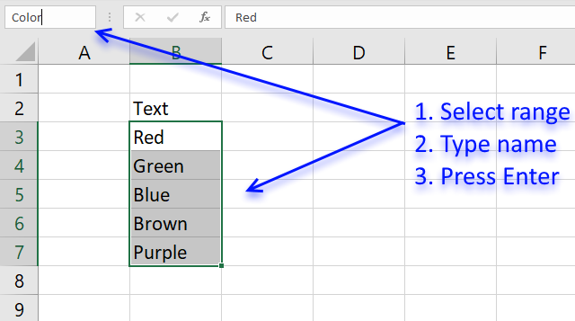
12.two.1 How to create a named range

The downside with named ranges is that you need to adjust the range every time you add together or delete a value in the list, the named range will then not fit the value list. I recommend using excel divers tables if you know that the list may change in the future.

1. Select cell range B3:B7
2. Type Colorin proper noun box
3. Press Enter

Formula example containing name range:

=Alphabetize(Color,Lucifer(0,COUNTIF($C$ii:C2,Color),0))

Back to top

xiii. How to remove errors (Excel 2007)

Excel 2007 users (and later versions) tin can remove errors using IFERROR() function.

When the formula runs out of values it returns #N/A errors (Non Available), you tin employ the IFERROR function to remove the mistake and render blanks in those cells.

Unfortunately, it comes with a big disadvantage, information technology as well removes other formula errors as well. So use this with cracking caution. If your source table has errors you won't detect it because the IFERROR part returns a blank cell instead.

Array formula in jail cell D2:

=IFERROR(LOOKUP(2, 1/(COUNTIF($D$2:D2, $B$3:$B$21)=0), $B$3:$B$21), "")

and re-create it down as far equally necessary.

Back to summit

Recommended articles

How to use the IFERROR function
How to use the ISERROR function
How to use the Mistake.TYPE function
How to notice errors in a worksheet
Delete blanks and errors in a list

Back to top

14. Excel 2003 users can remove errors using isna() function:

=IF(ISNA(Index($A$2:$A$xx, Friction match(0, COUNTIF($B$i:B1, $A$two:$A$20), 0))), "", INDEX($A$2:$A$20, MATCH(0, COUNTIF($B$i:B1, $A$ii:$A$20), 0)))

and copy it downwards equally far as needed.

This formula is an array formula, how to enter an array formula.

Recommended article

• ISNA function

Dorsum to tiptop

15. How to ignore blank cells in a range

Harlan Grove created a formula to count unique distinct values from a listing with blanks. I used the aforementioned technique here to filter unique distinct values in column D.

If y'all want a header name you can use the slightly larger formula, displayed in cavalcade F below.

Update 2020-12-09, Excel 365 users can use this regular formula:

=UNIQUE(FILTER($B$iii:$B$21, ($B$3:$B$21<>"") * ($B$3:$B$21<>"")))

The formula below is actually 58 graphic symbol while the new Excel 365 formula higher up is 61 characters, infinite characters not included. You tin notice a formula explanation here: Extract unique singled-out values ignoring blanks

Apply the formula beneath if you lot have an before Excel version than Excel 365.

Update 2017-09-01, smaller regular formula in jail cell D3:

=LOOKUP(ii, 1/(COUNTIF($D$ii:D2, $B$3:$B$21&"")=0), $B$iii:$B$21)

Formula in cell F3 if yous need a column header proper name:

=LOOKUP(two, 1/((COUNTIF($F$2:F2, $B$3:$B$21)+($B$3:$B$21=""))=0), $B$iii:$B$21)

fifteen.1 Sentry a video where I explain how these 2 formulas work

Subscribe to Get Digital Assist on Youtube:

This article shows y'all how to fill blank cells with values or formulas

Larn how to extract non-blank cells in a listing using a formula:

Remove blank cells

In this blog post I will provide two solutions on how to remove bare cells and a solution on how […]

Remove blank cells

Back to top

15.2 Get Excel file

Dorsum to tiptop

Source: https://www.get-digital-help.com/how-to-extract-a-unique-list-and-the-duplicates-in-excel-from-one-column/

Posted by: williamssaver1959.blogspot.com

Share this post