

How To Copy Data From One Excel Sheet To Another Using Vlookup
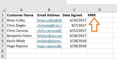
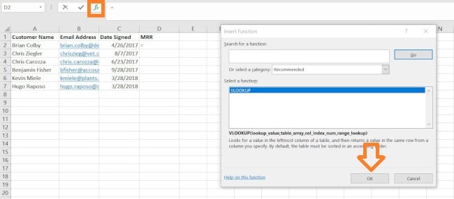
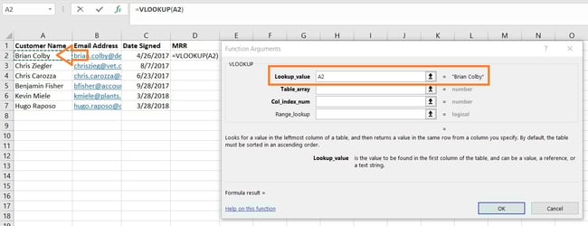
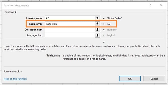
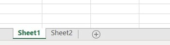
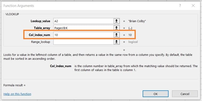
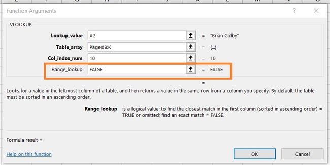
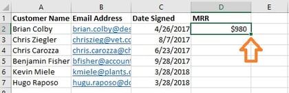
Analogous a massive amount of data in Microsoft Excel is a time-consuming headache. That headache can be fabricated even worse when you need to compare data across multiple spreadsheets. The final thing you want to practise is manually transfer cells using copy and paste. Thankfully, you don't have to. The VLOOKUP function tin can assistance you lot automate this task and salvage you tons of time. I know, "VLOOKUP office" sounds like the geekiest, most complicated affair ever. Simply past the fourth dimension you end reading this article, you'll wonder how you lot e'er survived in Excel without it. Microsoft Excel's VLOOKUP function is easier to utilise than you think. What's more, it is incredibly powerful, and is definitely something you want to have in your arsenal of belittling weapons. VLOOKUP stands for "vertical lookup." In Excel, this means the act of looking upwards data vertically across a spreadsheet, using the spreadsheet's columns -- and a unique identifier within those columns -- as the ground of your search. When you look upwardly your data, information technology must exist listed vertically wherever that data is located. When conducting a VLOOKUP in Excel, you're essentially looking for new data in a different spreadsheet that is associated with old data in your current i. When VLOOKUP runs this search, information technology e'er looks for the new information to the correct of your current data. For instance, if one spreadsheet has a vertical listing of names, and another spreadsheet has an unorganized list of those names and their electronic mail addresses, you can use VLOOKUP to retrieve those e-mail addresses in the order you lot have them in your first spreadsheet. Those email addresses must be listed in the column to the right of the names in the 2d spreadsheet, or Excel won't exist able to discover them. (Go effigy ... ) The secret to how VLOOKUP works? Unique identifiers. A unique identifier is a piece of information that both of your data sources share, and -- every bit its name implies -- information technology is unique (i.due east. the identifier is but associated with 1 record in your database). Unique identifiers include product codes, stock-keeping units (SKUs), and customer contacts. Alright, enough explanation: let'south see another instance of the VLOOKUP in activity! In the video beneath, we'll show an case in activeness, using the VLOOKUP part to match email addresses (from a 2d information source) to their corresponding data in a carve up sheet. Author's note: There are many different versions of Excel, so what yous see in the video above might not ever friction match upwardly exactly with what you'll come across in your version. That'due south why nosotros encourage you to follow along with the written instructions below. For your reference, here'due south what a VLOOKUP role looks similar: In the steps below, we'll assign the right value to each of these components, using customer names as our unique identifier to discover the MRR of each customer. Remember, y'all're looking to retrieve data from another sheet and eolith it into this one. With that in mind, label a column next to the cells you want more information on with a proper title in the meridian cell, such as "MRR," for monthly recurring revenue. This new column is where the data you're fetching will become. To the left of the text bar above your spreadsheet, you'll run into a small-scale function icon that looks like a script: Fx. Click on the first empty cell below your column title and then click this function icon. A box titled Formula Architect or Insert Office will appear to the right of your screen (depending on which version of Excel yous take). Search for and select "VLOOKUP" from the list of options included in the Formula Builder. Then, select OK or Insert Function to first building your VLOOKUP. The cell yous currently have highlighted in your spreadsheet should at present look similar this: "=VLOOKUP()" Yous can also enter this formula into a call manually by entering the bold text above exactly into your desired cell. With the =VLOOKUP text entered into your starting time prison cell, it's fourth dimension to fill the formula with iv different criteria. These criteria volition assistance Excel narrow downward exactly where the data you want is located and what to look for. The first criteria is your lookup value -- this is the value of your spreadsheet that has information associated with it, which you lot want Excel to discover and return for you lot. To enter it, click on the prison cell that carries a value yous're trying to find a friction match for. In our example, shown higher up, it'southward in prison cell A2. You'll start migrating your new data into D2, since this cell represents the MRR of the client proper name listed in A2. Continue in mind your lookup value can exist anything: text, numbers, website links, you proper noun it. As long as the value yous're looking up matches the value in the referring spreadsheet -- which we'll talk most that in the side by side stride -- this function will render the data you lot want. Next to the "table array" field, enter the range of cells you'd like to search and the sheet where these cells are located, using the format shown in the screenshot above. The entry above means the data nosotros're looking for is in a spreadsheet titled "Pages" and can be found anywhere betwixt column B and column Thou. The sail where your data is located must be within your current Excel file. This means your data can either be in a different tabular array of cells somewhere in your electric current spreadsheet, or in a different spreadsheet linked at the bottom of your workbook, as shown below. For example, if your data is located in "Sheet2" between cells C7 and L18, your table array entry will be "Sheet2!C7:L18." Beneath the table assortment field, yous'll enter the "column alphabetize number" of the table array yous're searching through. For case, if you're focusing on columns B through K (notated "B:K" when entered in the "tabular array assortment" field), but the specific values y'all desire are in column K, you'll enter "10" in the "column index number" field, since column Thousand is the tenth column from the left. In situations like ours, which concerns monthly revenue, you want to find verbal matches from the table yous're searching through. To do this, enter "Simulated" in the "range lookup" field. This tells Excel y'all want to observe only the exact revenue associated with each sales contact. To reply your called-for question: Yes, you can let Excel to look for an approximate match instead of an exact friction match. To do so, simply enter TRUE instead of Simulated in the fourth field shown above. When VLOOKUP is fix for an gauge lucifer, it's looking for data that almost closely resembles your lookup value, rather than data that is identical to that value. If you're looking up data associated with a listing of website links, for case, and some of your links accept "https://" at the beginning, it might behoove y'all to find an approximate match simply in case at that place are links that practise not accept this "https://" tag. This fashion, the rest of the link can match without this initial text tag causing your VLOOKUP formula to return an error if Excel tin can't find information technology. In club to officially bring in the values you want into your new column from Stride one, click "Done" (or "Enter," depending on your version of Excel) later filling the "range lookup" field. This will populate your start prison cell. You might accept this opportunity to look in the other spreadsheet to make sure this was the correct value. If so, populate the rest of the new column with each subsequent value by clicking the get-go filled cell, then clicking the tiny square that appears on the lesser-right corner of this prison cell. Washed! All your values should appear. If you've followed the higher up steps and your VLOOKUP is yet not working, it will either be an issue with your: Start with looking at the VLOOKUP formula that yous have written in the designated cell. If the syntax is not the trouble, how you may have an issue with the values you're trying to receive themselves. This often manifests every bit an #N/A mistake where the VLOOKUP cannot find a referenced value. For example, if y'all're looking up URL data, each URL must exist a row with its corresponding data to the left of it in the same row. If you take the URLs every bit column headers with the data moving vertically, the VLOOKUP volition non work. Keeping with this example, the URLs must match in format in both sheets. If you accept 1 sheet including the "https://" in the value while the other sheet omits the "https://", the VLOOKUP will not be able to lucifer the values. Marketers take to analyze information from a diverseness of sources to get a complete picture of pb generation (and more). Microsoft Excel is the perfect tool to practice this accurately and at calibration, particularly with the VLOOKUP function. Editor'south note: This postal service was originally published in March 2019 and has been updated for comprehensiveness. ![Download 10 Excel Templates for Marketers [Free Kit]](https://no-cache.hubspot.com/cta/default/53/9ff7a4fe-5293-496c-acca-566bc6e73f42.png) What does VLOOKUP exercise, exactly? Here'south the unproblematic explanation: The VLOOKUP function searches for a specific value in your data, and in one case it identifies that value, information technology can notice -- and display -- some other slice of information that's associated with that value.
What does VLOOKUP exercise, exactly? Here'south the unproblematic explanation: The VLOOKUP function searches for a specific value in your data, and in one case it identifies that value, information technology can notice -- and display -- some other slice of information that's associated with that value.How does VLOOKUP work?
The formula always searches to the right.
The formula needs a unique identifier to retrieve data.
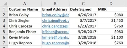
VLOOKUP Example
How to Use VLOOKUP in Excel
VLOOKUP(lookup_value , table_array , col_index_num , range_lookup)
1. Place a cavalcade of cells you'd like to fill with new information.
2. Select 'Function' (Fx) > VLOOKUP and insert this formula into your highlighted cell.
3. Enter the lookup value for which you want to retrieve new information.
iv. Enter the table assortment of the spreadsheet where your desired information is located.
5. Enter the cavalcade number of the data you want Excel to render.
6. Enter your range lookup to discover an exact or judge match of your lookup value.
7. Click 'Done' (or 'Enter') and fill your new column.
VLOOKUP Not Working?
Troubleshooting VLOOKUP Syntax
Troubleshooting VLOOKUP Values
VLOOKUPs equally a Powerful Marketing Tool


Originally published Jul 14, 2021 1:15:00 PM, updated July 14 2021

Source: https://blog.hubspot.com/marketing/vlookup-excel
Posted by: williamssaver1959.blogspot.com
0 Response to "How To Copy Data From One Excel Sheet To Another Using Vlookup"
Post a Comment